In-Class Exercise 2B: Global and Local Spatial Autocorrelations

Using sfdep package

Author

Goh Si Hui

Published

November 25, 2023

Modified

November 27, 2023

1 Overview

For this task, we will be learning how to compute global and local spatial autocorrelations using the sfdep package.

2 Getting Started

We will first load the necessary packages using the following code chunk:

tmap: for thematic mapping
sf: for geospatial data handling (e.g. importing and exporting for spatial data and geoprocessing)
tidyverse: a family of R packages for non-spatial data handling
knitr: to generate static html tables
sfdep: to calculate spatial weights and matrices, space time cube and hot spot analysis
plotly: to make the graphs interactive

pacman::p_load(tmap, sf, tidyverse, sfdep, knitr, plotly)

3 Preparing the Geospatial Data

3.1 Importing the data

hunan <- st_read(dsn = "data/geospatial", layer="Hunan")

Reading layer `Hunan' from data source 
  `C:\sihuihui\ISSS624\In-class_Ex\In-class_Ex2\data\geospatial' 
  using driver `ESRI Shapefile'
Simple feature collection with 88 features and 7 fields
Geometry type: POLYGON
Dimension:     XY
Bounding box:  xmin: 108.7831 ymin: 24.6342 xmax: 114.2544 ymax: 30.12812
Geodetic CRS:  WGS 84

From the above outcome, we know that hunandata is simple feature (sf) data frame with 88 features (each representing 1 geographical entity), and each feature is a polygon.It uses the WGS84 projection.

4 Preparing the Aspatial Data

4.1 Importing the data

hunan2012 <- read.csv("data/aspatial/Hunan_2012.csv")

5 Combining Both Data Frames Using Left Join

hunan_GDPPC<- left_join(hunan, hunan2012) %>% 
                select(1:4, 7, 15)

When joining these 2 data frames, we did not specify the by= because there is a common column in both data frames (i.e., Country )

Other than joining both data frames, we also use select() to pick the relevant columns that we want. Note that the geometry column was retained even though it was not specified.

We typically use a left join with a spatial layer (e.g. hunan) and nonspatial layer (hunan_GDPPC) so that we can retain spatial geometric properties.

6 Plotting the Choropleth Map

We use the following code to visualise the choropleth map of Hunan’s 2012 GDPPC.

tmap_mode("plot")
tm_shape(hunan_GDPPC) +
  tm_fill("GDPPC",
          style = "quantile",
          palette = "Blues",
          title = "GDPPC") + 
  tm_borders(alpha = 0.5) + 
  tm_layout(main.title = "Distribution of GDP per capita by district in Hunan (2012)", main.title.position="center",
            main.title.size=0.8,
            legend.height = 0.45,
            legend.width = 0.35, 
            frame= TRUE) +
  tm_compass(type = "8star", size=2) +
  tm_scale_bar() +
  tm_grid(alpha = 0.2)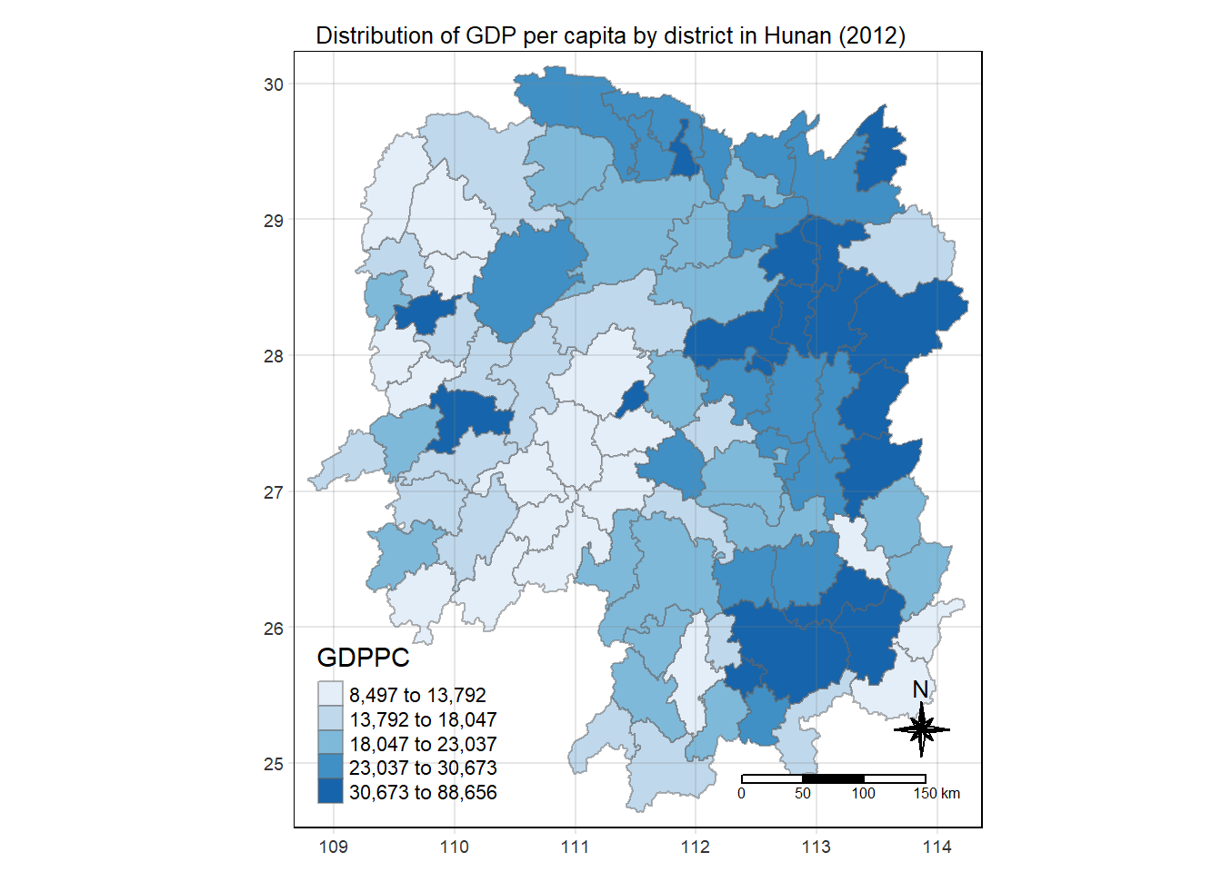

7 Global Measures of Spatial Association

7.1 Deriving Contiguity Weights (Queen’s Method)

The following code chunk derives the Queen’s method contiguity weights.

wm_q <- hunan_GDPPC %>%
  mutate(nb = st_contiguity(geometry), 
         wt = st_weights(nb, 
                         style = "W"),
         .before = 1)

Explanation of the function(s) used above

st_weights() provides 3 arguments:
- nb: a neighbour list object as creatd by st_neighbours()
- style: Default is “W” for row standardised weights. This value can also be “B”, “C”, “U”, “minmax”, and “S”. B is the basic binary coding, W is row standardised (sums over all links to n), C is globally standardised (sums over all links to n), U is equal to C divided by the number of neighbours (sums over all links to unity), while S is the variance-stabilizing coding scheme proposed by Tiefelsdorf et al. 1999, p. 167-168 (sums over all links to n).
- allow_zero: If TRUE, it assigns zero as lagged value to zone without neighbours.

Let us take a look at the data frame generated.

wm_q

Simple feature collection with 88 features and 8 fields
Geometry type: POLYGON
Dimension:     XY
Bounding box:  xmin: 108.7831 ymin: 24.6342 xmax: 114.2544 ymax: 30.12812
Geodetic CRS:  WGS 84
First 10 features:
                               nb
1                 2, 3, 4, 57, 85
2               1, 57, 58, 78, 85
3                     1, 4, 5, 85
4                      1, 3, 5, 6
5                     3, 4, 6, 85
6                4, 5, 69, 75, 85
7                  67, 71, 74, 84
8       9, 46, 47, 56, 78, 80, 86
9           8, 66, 68, 78, 84, 86
10 16, 17, 19, 20, 22, 70, 72, 73
                                                                            wt
1                                                      0.2, 0.2, 0.2, 0.2, 0.2
2                                                      0.2, 0.2, 0.2, 0.2, 0.2
3                                                       0.25, 0.25, 0.25, 0.25
4                                                       0.25, 0.25, 0.25, 0.25
5                                                       0.25, 0.25, 0.25, 0.25
6                                                      0.2, 0.2, 0.2, 0.2, 0.2
7                                                       0.25, 0.25, 0.25, 0.25
8  0.1428571, 0.1428571, 0.1428571, 0.1428571, 0.1428571, 0.1428571, 0.1428571
9             0.1666667, 0.1666667, 0.1666667, 0.1666667, 0.1666667, 0.1666667
10                      0.125, 0.125, 0.125, 0.125, 0.125, 0.125, 0.125, 0.125
     NAME_2  ID_3    NAME_3   ENGTYPE_3    County GDPPC
1   Changde 21098   Anxiang      County   Anxiang 23667
2   Changde 21100   Hanshou      County   Hanshou 20981
3   Changde 21101    Jinshi County City    Jinshi 34592
4   Changde 21102        Li      County        Li 24473
5   Changde 21103     Linli      County     Linli 25554
6   Changde 21104    Shimen      County    Shimen 27137
7  Changsha 21109   Liuyang County City   Liuyang 63118
8  Changsha 21110 Ningxiang      County Ningxiang 62202
9  Changsha 21111 Wangcheng      County Wangcheng 70666
10 Chenzhou 21112     Anren      County     Anren 12761
                         geometry
1  POLYGON ((112.0625 29.75523...
2  POLYGON ((112.2288 29.11684...
3  POLYGON ((111.8927 29.6013,...
4  POLYGON ((111.3731 29.94649...
5  POLYGON ((111.6324 29.76288...
6  POLYGON ((110.8825 30.11675...
7  POLYGON ((113.9905 28.5682,...
8  POLYGON ((112.7181 28.38299...
9  POLYGON ((112.7914 28.52688...
10 POLYGON ((113.1757 26.82734...

7.2 Computing Global Moran’s I

In the code chunk below, global_moran() function is used to compute the Moran’s I value. Different from spdep package, the output is a tibble data.frame.

moranI <- global_moran(wm_q$GDPPC,
                       wm_q$nb,
                       wm_q$wt)

glimpse(moranI)

List of 2
 $ I: num 0.301
 $ K: num 7.64

7.3 Performing Global Moran’s I test

In general, Moran’s I test will be performed instead of just computing the Moran’s I statistics. With sfdep package, Moran’s I test can be performed by using global_moran_test() as shown in the code chunk below.

global_moran_test(wm_q$GDPPC, 
                  wm_q$nb,
                  wm_q$wt)


    Moran I test under randomisation

data:  x  
weights: listw    

Moran I statistic standard deviate = 4.7351, p-value = 1.095e-06
alternative hypothesis: greater
sample estimates:
Moran I statistic       Expectation          Variance 
      0.300749970      -0.011494253       0.004348351

Note

The default for alternative argument is “two.sided”. Other supported arguments are “greater” or “less”.
By default, the randomizaton argument is TRUE. If FALSE, it assumes normality.

7.4 Performning Global Moran’s I permutation test

In practice, monte carlo simulation should be used to perform the statistical test. For sfdep, it is supported by globel_moran_perm().

Note

It is a good practice to use set.seed() before performing simulation. This is to ensure that the computation is reproducible.

set.seed(1234)
global_moran_perm(wm_q$GDPPC,
                  wm_q$nb,
                  wm_q$wt, 
                  nsim=99)


    Monte-Carlo simulation of Moran I

data:  x 
weights: listw  
number of simulations + 1: 100 

statistic = 0.30075, observed rank = 100, p-value < 2.2e-16
alternative hypothesis: two.sided

Since the p value is <2.2e-16, which is lower than the significance level of 0.05, we can reject the null hypothesis that the spatial patterns are random. Because the Moran’s I statistic is greater than 0, we can infer that the spatial distribution shows signs of clustering.

Note

The numbers of simulation is alway equal to nsim + 1. This mean in nsim = 99. This mean 100 simulation will be performed.

7.5 Computing Local Moran’s I

We can compute Local Moran’s I of GDPPC at county level using local_moran() of sfdep package.

lisa <- wm_q %>% 
  mutate(local_moran = local_moran(GDPPC, nb, wt, nsim = 99),
         .before=1) %>% 
  unnest(local_moran)

Let us take a look at the output.

lisa

Simple feature collection with 88 features and 20 fields
Geometry type: POLYGON
Dimension:     XY
Bounding box:  xmin: 108.7831 ymin: 24.6342 xmax: 114.2544 ymax: 30.12812
Geodetic CRS:  WGS 84
# A tibble: 88 × 21
         ii        eii     var_ii    z_ii    p_ii p_ii_sim p_folded_sim skewness
      <dbl>      <dbl>      <dbl>   <dbl>   <dbl>    <dbl>        <dbl>    <dbl>
 1 -0.00147  0.00177   0.000418   -0.158  0.874       0.82         0.41   -0.812
 2  0.0259   0.00641   0.0105      0.190  0.849       0.96         0.48   -1.09 
 3 -0.0120  -0.0374    0.102       0.0796 0.937       0.76         0.38    0.824
 4  0.00102 -0.0000349 0.00000437  0.506  0.613       0.64         0.32    1.04 
 5  0.0148  -0.00340   0.00165     0.449  0.654       0.5          0.25    1.64 
 6 -0.0388  -0.00339   0.00545    -0.480  0.631       0.82         0.41    0.614
 7  3.37    -0.198     1.41        3.00   0.00266     0.08         0.04    1.46 
 8  1.56    -0.265     0.804       2.04   0.0417      0.08         0.04    0.459
 9  4.42     0.0450    1.79        3.27   0.00108     0.02         0.01    0.746
10 -0.399   -0.0505    0.0859     -1.19   0.234       0.28         0.14   -0.685
# ℹ 78 more rows
# ℹ 13 more variables: kurtosis <dbl>, mean <fct>, median <fct>, pysal <fct>,
#   nb <nb>, wt <list>, NAME_2 <chr>, ID_3 <int>, NAME_3 <chr>,
#   ENGTYPE_3 <chr>, County <chr>, GDPPC <int>, geometry <POLYGON [°]>

The output of local_moran() is an sf data.frame containing the columns ii, eii, var_ii, z_ii, p_ii, p_ii_sim, p_folded_sim, skewness and kurtosis.

ii: local moran statistic
eii: expectation of local moran statistic; for localmoran_perm(), it refers to the permutation sample means
var.ii:variance of local moran statistic; for localmoran_perm(), it refers to the permutation sample standard deviations
z_ii: standard deviate of local moran statistic; for localmoran_perm(), based on permutation sample means and standard deviations
p_ii:p-value of local moran statistic using pnorm(); for localmoran_perm() using standard
p_ii_sim: For localmoran_perm(), rank() and punif() of observed statistic rank for [0, 1] p-values using alternative=
p_folded_sim: the simulation folded [0, 0.5] range ranked p-value (based on this)
skewness: For localmoran_perm(), the output of e1071::skewness() for the permutation samples underlying the standard deviates
Kurtosis: For localmoran_perm(), the output of e1071::kurtosis() for the permutation samples underlying the standard deviates

7.6 Visualising Local Moran’s I

We can use tmap package to prepare a choropleth map using the values in the ii field.

tmap_mode("plot")
tm_shape(lisa) +
  tm_fill("ii") +
  tm_borders(alpha = 0.5) +
  tm_view(set.zoom.limits = c(6,8)) +
  tm_layout(main.title = "Local Moran's I of GDPPC", 
            main.title.size = 0.8)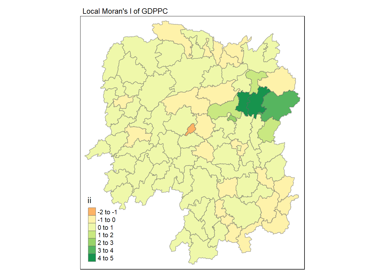

7.7 Visualising Local Moran’s p-values

We can use tmap package to prepare a choropleth map using the values in the p_ii field.

tmap_mode("plot")
tm_shape(lisa) +
  tm_fill("p_ii", breaks = c(0, 0.001, 0.01, 0.05, 1),
              labels = c("0.001", "0.01", "0.05", "Not sig")) +
  tm_borders(alpha = 0.5) +
  tm_layout(main.title = "p-value of Local Moran's I", 
            main.title.size = 0.8)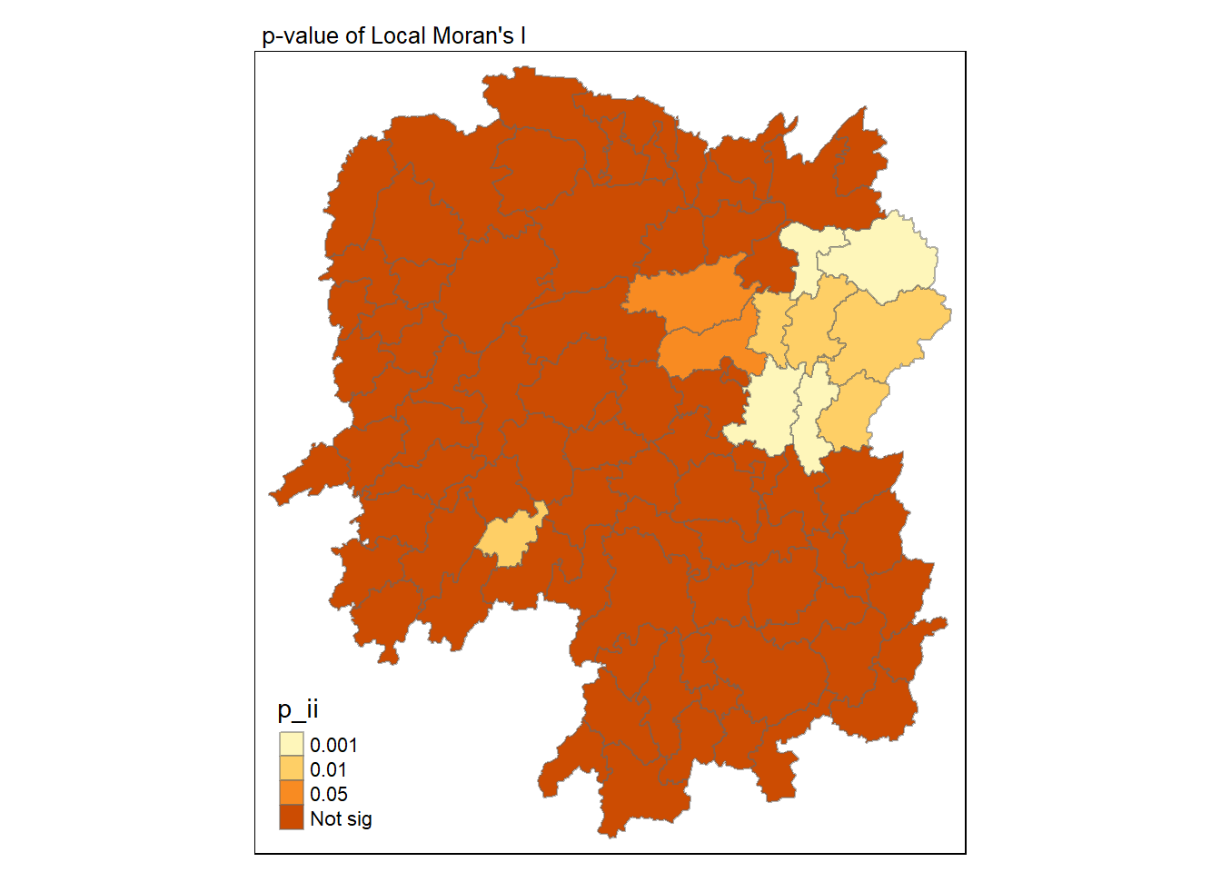

7.8 Visualising Local Moran’s I and p-values

For effective comparison, let us plot both maps next to each other.

tmap_mode("plot")
ii_val <- tm_shape(lisa) +
  tm_fill("ii") +
  tm_borders(alpha = 0.5) +
  tm_view(set.zoom.limits = c(6,8)) +
  tm_layout(main.title = "Local Moran's I of GDPPC", 
            main.title.size = 0.8)

pii_val <- tm_shape(lisa) +
  tm_fill("p_ii", breaks = c(0, 0.001, 0.01, 0.05, 1),
              labels = c("0.001", "0.01", "0.05", "Not sig")) +
  tm_borders(alpha = 0.5) +
  tm_layout(main.title = "p-value of Local Moran's I", 
            main.title.size = 0.8)

tmap_arrange(ii_val, pii_val, asp = 1, ncol = 2)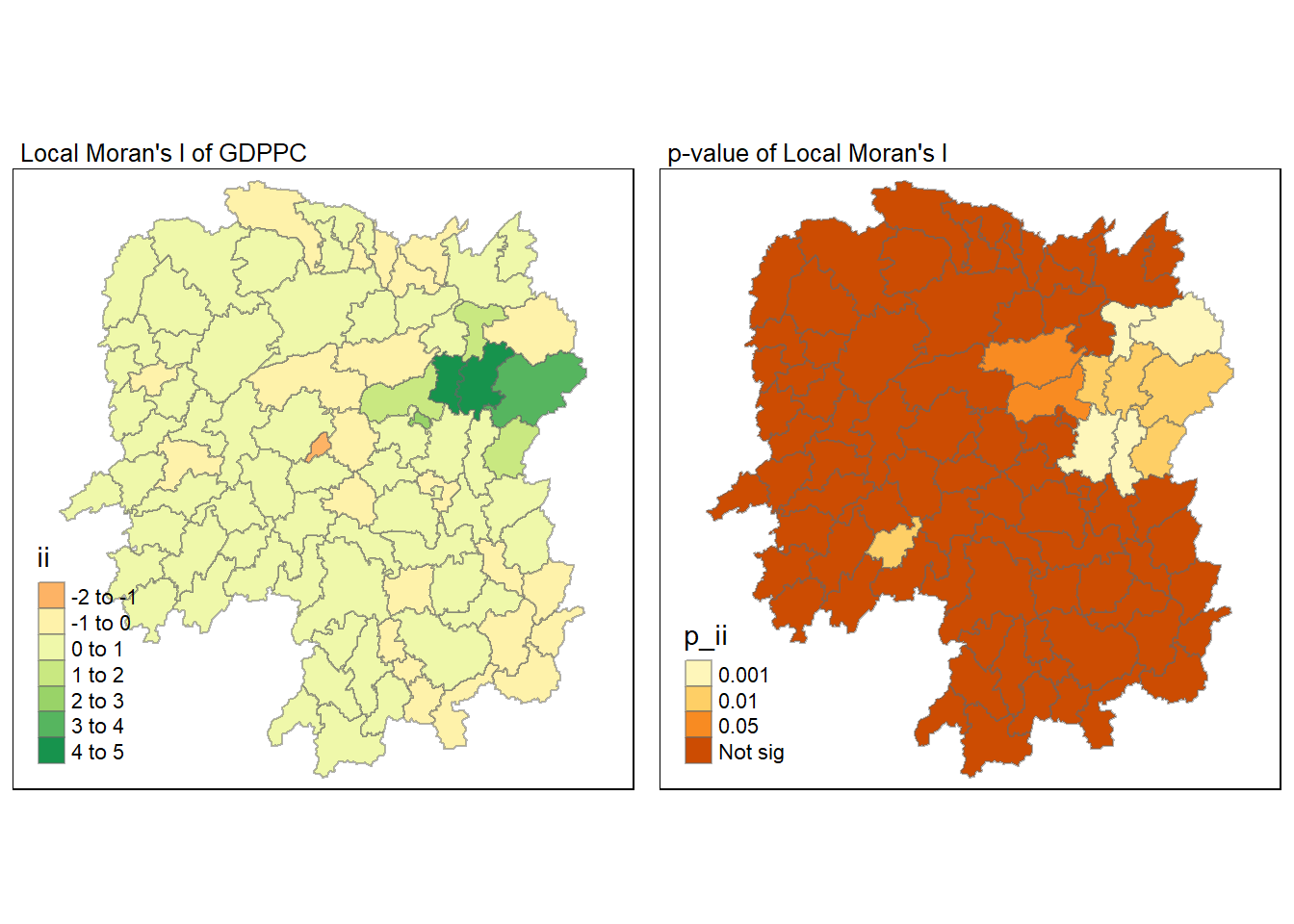

7.9 Visualising LISA Map

LISA map is a categorical map showing outliers and clusters. There are two types of outliers namely: High-Low and Low-High outliers. Likewise, there are two type of clusters namely: High-High and Low-Low cluaters. In fact, LISA map is an interpreted map by combining local Moran’s I of geographical areas and their respective p-values.

In lisa sf data.frame, we can find three fields contain the LISA categories. They are mean, median and pysal. In general, classification in mean will be used as shown in the code chunk below.

lisa_sig <- lisa %>% 
  filter(p_ii <0.05)

tmap_mode("plot")
tm_shape(lisa) + 
  tm_polygons() +
  tm_borders(alpha = 0.5) +
  tm_shape(lisa_sig) + 
  tm_fill("mean") +
  tm_borders(alpha = 0.4)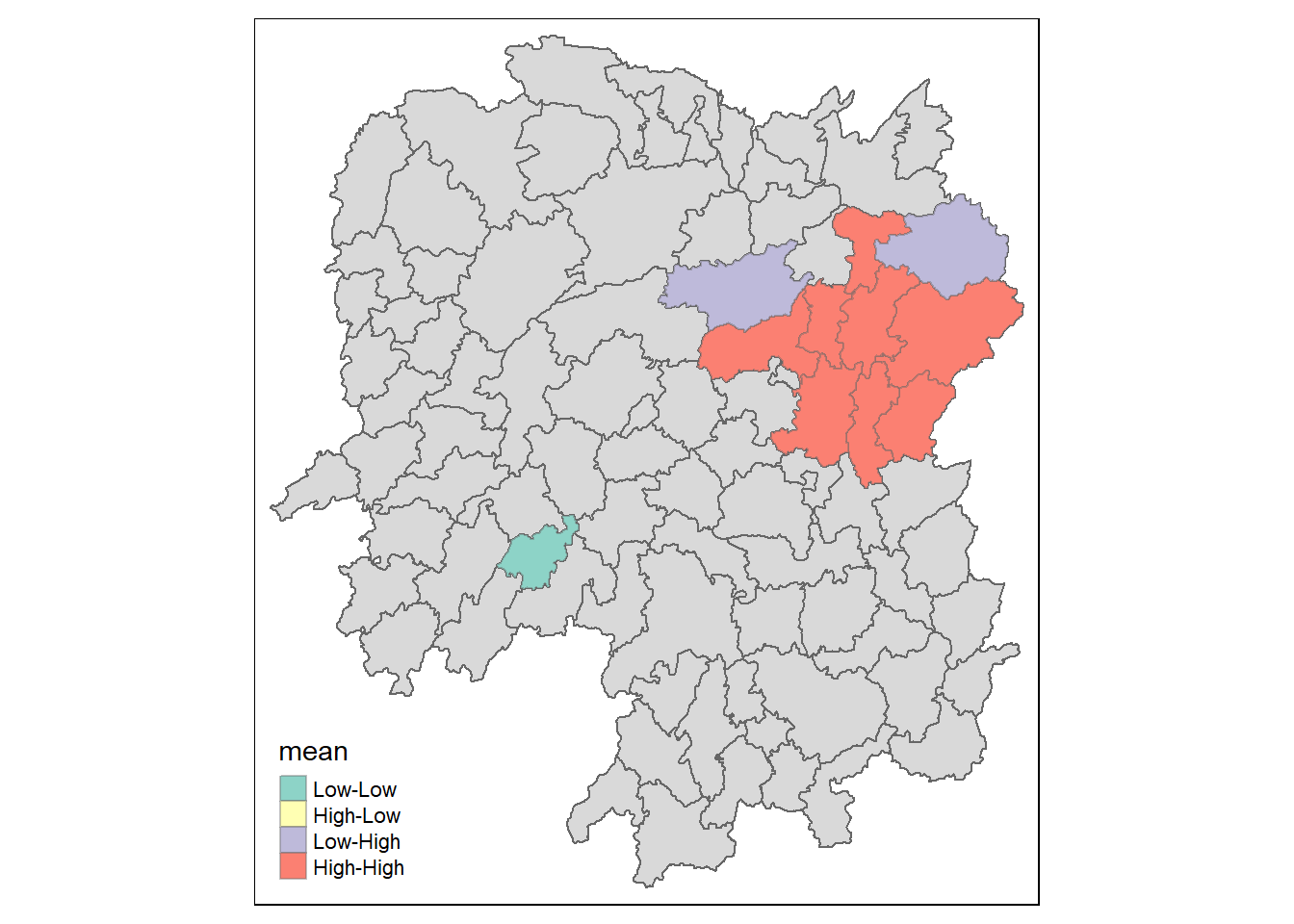

8 Hot Spot and Cold Spot Area Analysis (HCSA)

HCSA uses spatial weights to identify locations of statistically significant hot spots and cold spots in an spatially weighted attribute that are in proximity to one another based on a calculated distance. The analysis groups features when similar high (hot) or low (cold) values are found in a cluster. The polygon features usually represent administration boundaries or a custom grid structure.

9 Computing local Gi* Statistics

First, we will compute an inverse distance weight matrix.

wm_idw <- hunan_GDPPC %>%
  mutate(nb = st_contiguity(geometry), 
         wt = st_inverse_distance(nb, geometry, 
                                  scale = 1,
                                  alpha = 1),
         .before=1)

We will then use local_gstar_perm() of sfdep package to compute local Gi* statistics using the following code chunk.

HCSA <- wm_idw %>% 
  mutate(local_Gi = local_gstar_perm(GDPPC, nb, wt, nsim=99),
         .before = 1) %>% 
  unnest(local_Gi)

Let us take a look at the output.

HCSA

Simple feature collection with 88 features and 16 fields
Geometry type: POLYGON
Dimension:     XY
Bounding box:  xmin: 108.7831 ymin: 24.6342 xmax: 114.2544 ymax: 30.12812
Geodetic CRS:  WGS 84
# A tibble: 88 × 17
   gi_star   e_gi    var_gi p_value   p_sim p_folded_sim skewness kurtosis nb   
     <dbl>  <dbl>     <dbl>   <dbl>   <dbl>        <dbl>    <dbl>    <dbl> <nb> 
 1  0.0416 0.0114   6.41e-6  0.0493 9.61e-1         0.7      0.35    0.875 <int>
 2 -0.333  0.0106   3.84e-6 -0.0941 9.25e-1         1        0.5     0.661 <int>
 3  0.281  0.0126   7.51e-6 -0.151  8.80e-1         0.9      0.45    0.640 <int>
 4  0.411  0.0118   9.22e-6  0.264  7.92e-1         0.6      0.3     0.853 <int>
 5  0.387  0.0115   9.56e-6  0.339  7.34e-1         0.62     0.31    1.07  <int>
 6 -0.368  0.0118   5.91e-6 -0.583  5.60e-1         0.72     0.36    0.594 <int>
 7  3.56   0.0151   7.31e-6  2.61   9.01e-3         0.06     0.03    1.09  <int>
 8  2.52   0.0136   6.14e-6  1.49   1.35e-1         0.2      0.1     1.12  <int>
 9  4.56   0.0144   5.84e-6  3.53   4.17e-4         0.04     0.02    1.23  <int>
10  1.16   0.0104   3.70e-6  1.82   6.86e-2         0.12     0.06    0.416 <int>
# ℹ 78 more rows
# ℹ 8 more variables: wt <list>, NAME_2 <chr>, ID_3 <int>, NAME_3 <chr>,
#   ENGTYPE_3 <chr>, County <chr>, GDPPC <int>, geometry <POLYGON [°]>

From the above results, we see that the following columns are generated due to local_gstar_perm() :

gi_star: the observed statistic
e_gi: the permutation sample mean
var_gi: the permutation sample variance
p_value: the p-value using sample mean and standard deviation
p_folded_sim: p-value based on the implementation of Pysal which always assumes a two-sided test taking the minimum possible p-value
skewness: sample skewness
kurtosis: sample kurtosis

9.1 Visualing Gi*

We use the following code chunk to visualise the Gi* computed.

tmap_mode("plot")

tm_shape(HCSA) +
  tm_fill("gi_star") +
  tm_borders(alpha = 0.5) +
  tm_view(set.zoom.limits = c(6,8))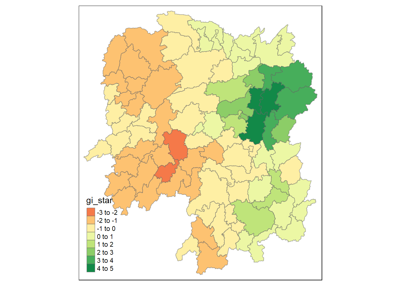

Visualising p-value of HCSA

We use the following code chunk to visualise the p-values of HCSA computed.

tmap_mode("plot")

tm_shape(HCSA) +
  tm_fill("p_folded_sim") +
  tm_borders(alpha = 0.5) +
  tm_view(set.zoom.limits = c(6,8))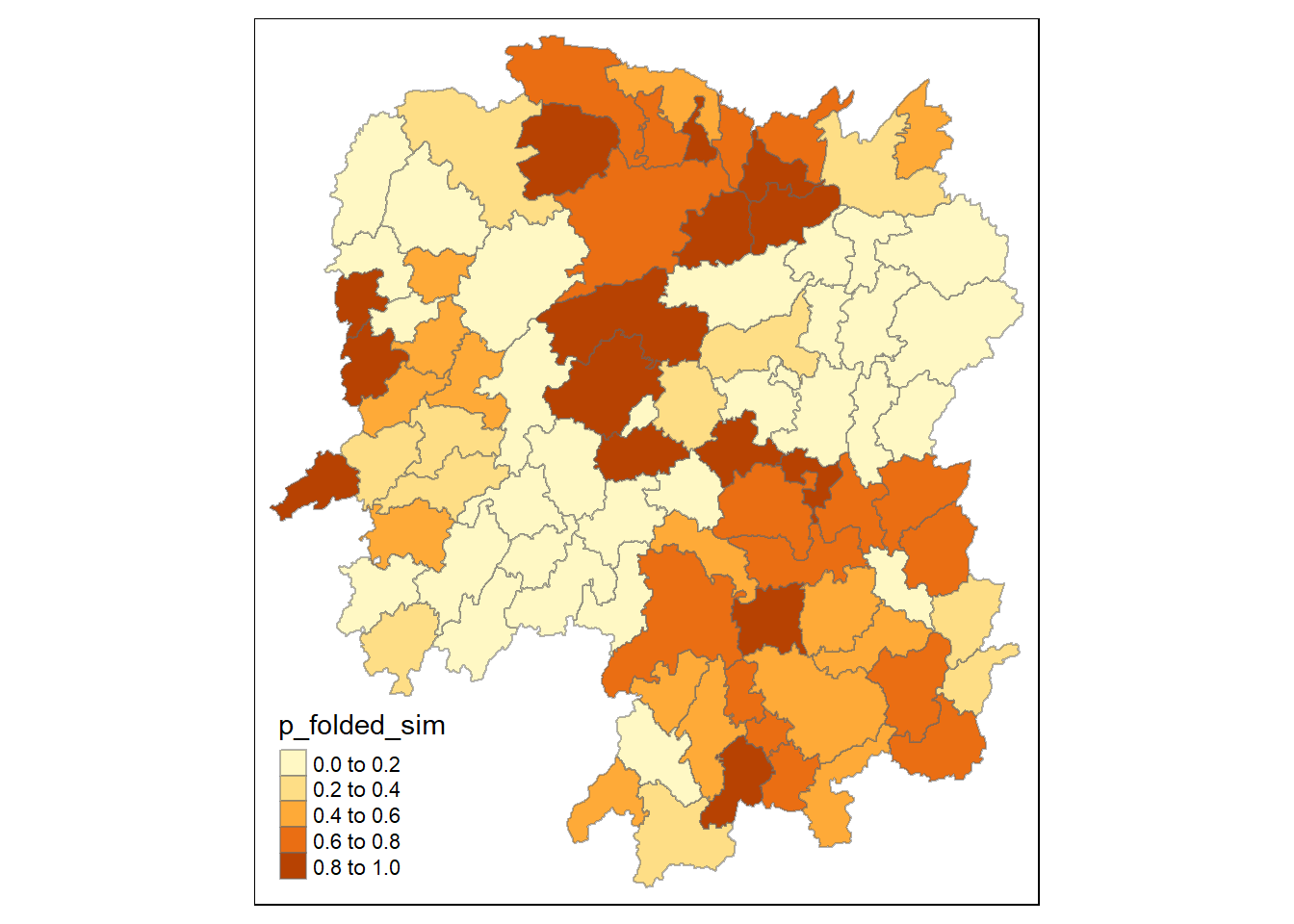

For effective comparison, we plot both maps next to each other.

tmap_mode("plot")
map1 <- tm_shape(HCSA) +
  tm_fill("gi_star") + 
  tm_borders(alpha = 0.5) +
  tm_view(set.zoom.limits = c(6,8)) +
  tm_layout(main.title = "Gi* of GDPPC",
            main.title.size = 0.8)

map2 <- tm_shape(HCSA) +
  tm_fill("p_value",
          breaks = c(0, 0.001, 0.01, 0.05, 1),
          labels = c("0.001", "0.01", "0.05", "Not sig")) + 
  tm_borders(alpha = 0.5) +
  tm_layout(main.title = "p-value of Gi*",
            main.title.size = 0.8)

tmap_arrange(map1, map2, ncol = 2)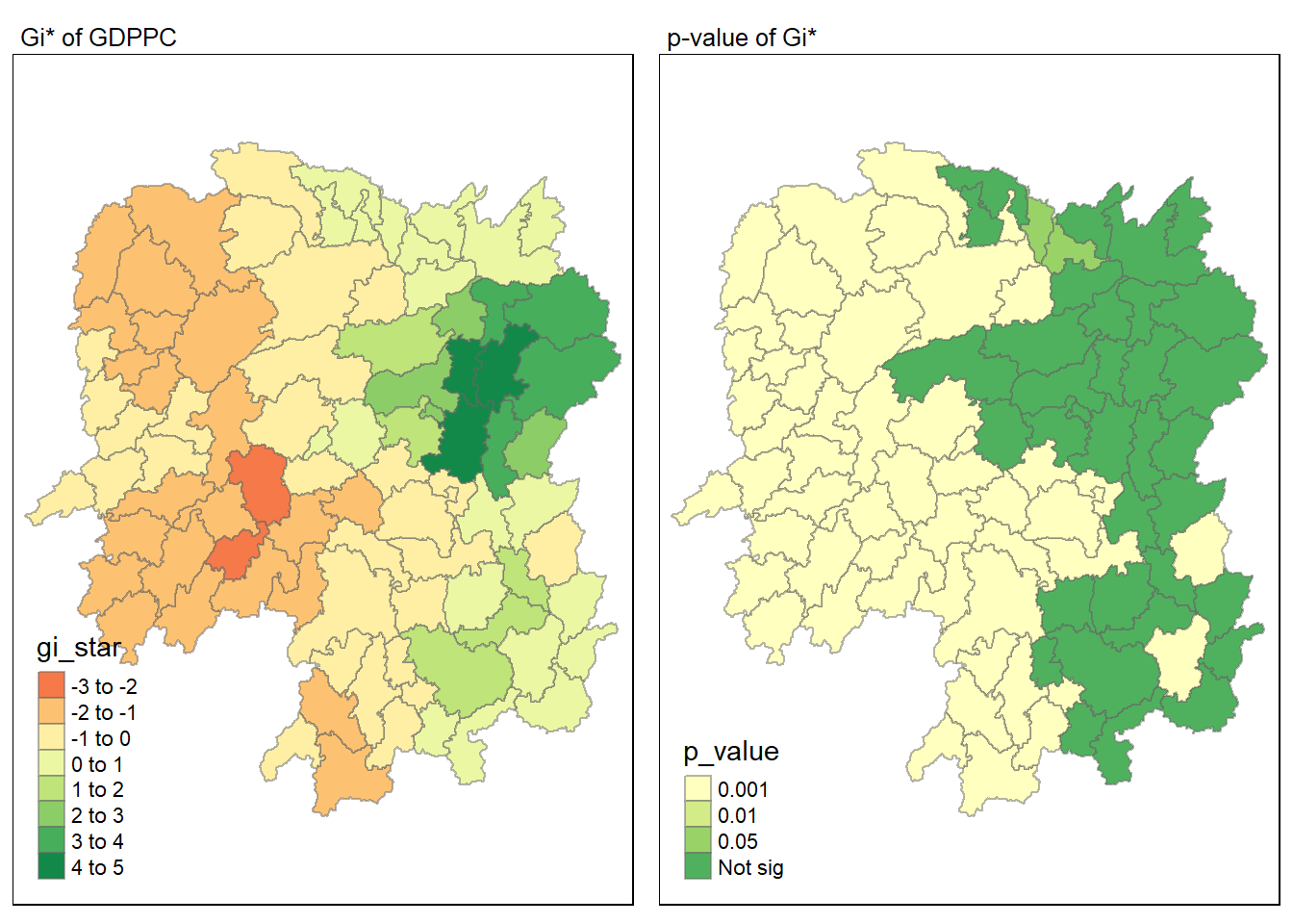

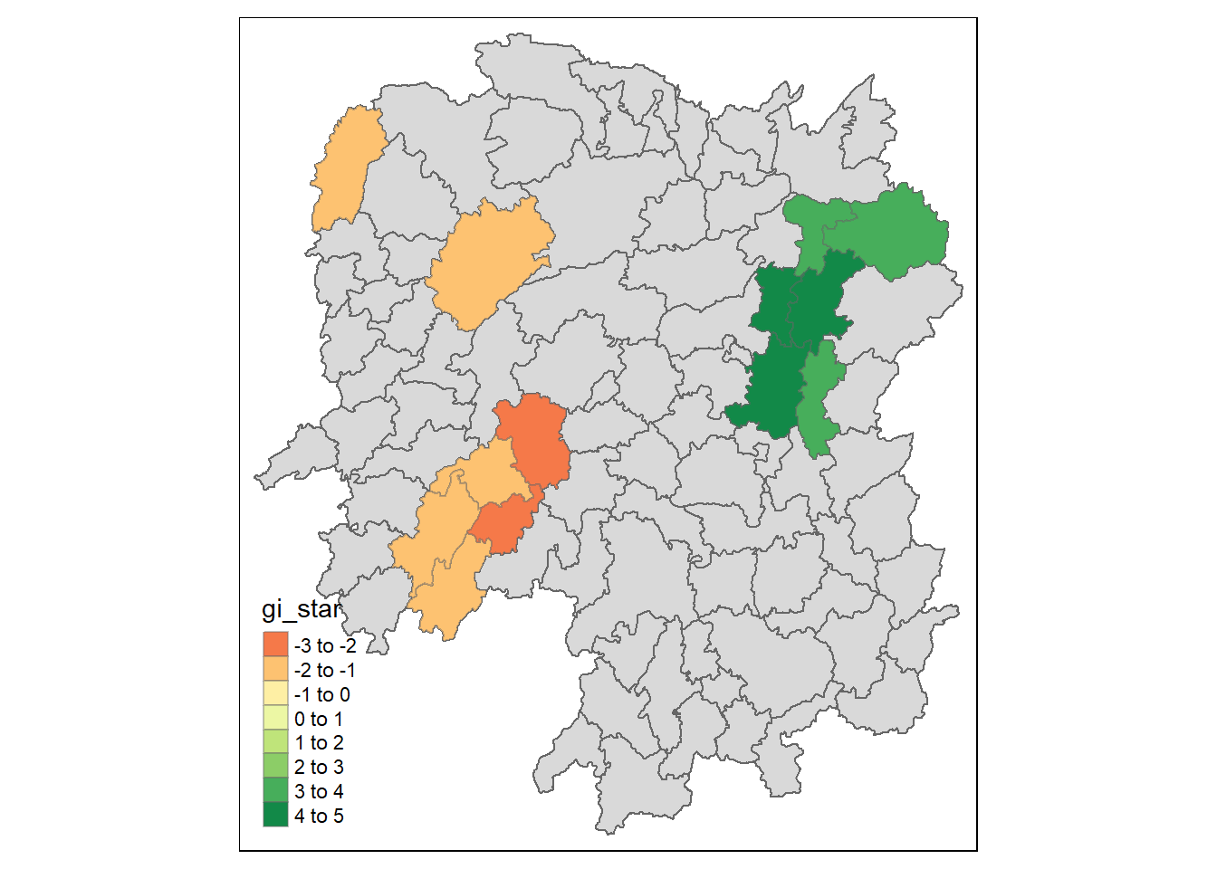
9.2 Visualising Hot Spot and Cold Spot Areas

Now, we are ready to plot the significant (i.e. p-values less than 0.05) hot spot and cold spot areas by using the following code chunk.

HCSA_sig <- HCSA  %>%
  filter(p_folded_sim < 0.05)

tmap_mode("plot")
tm_shape(HCSA) +
  tm_polygons() +
  tm_borders(alpha = 0.5) +
tm_shape(HCSA_sig) +
  tm_fill("gi_star") + 
  tm_borders(alpha = 0.4)